Blog Post | Stylianos Kyriacou

On “Randomly Wired” and “Optimally Wired” Feed Forward Neural Networks — Part 1

Author: Stylianos Kyriacou

Inspired by the recent publication of FAIR (https://arxiv.org/abs/1904.01569) were it has been reported that randomly wired NNs outperform all existing manually wired ones, such as ResNet, ShuffleNet, etc., at the ImageNet classification task this series of blog posts will examine:
a) the Randomly wired NNs (RWNNs) performance as they are applied on a “simple” regression case;
b) The use of an ensemble of RWNNs (with each ensemble member utilizing a different randomly generated architecture) to quantify prediction uncertainty (hopefully we’ll see uncertainty rise in extrapolation regions);
c) The use of an Evolutionary Algorithm (EA) to optimally wire a Neural Network (OWNN). This will include a single objective optimization were the OWNN wiring will be designed to maximize prediction accuracy (minimize training set prediction error); a bi-objective optimization problem were the OWNN will be designed to maximize prediction accuracy but also maximize the models generalization (error on test set) and a tri-objective problem were the minimization of the number of synapses will also be added as a third objective.

Randomly wired NNs (RWNNs) performance as they are applied on a “simple” regression case

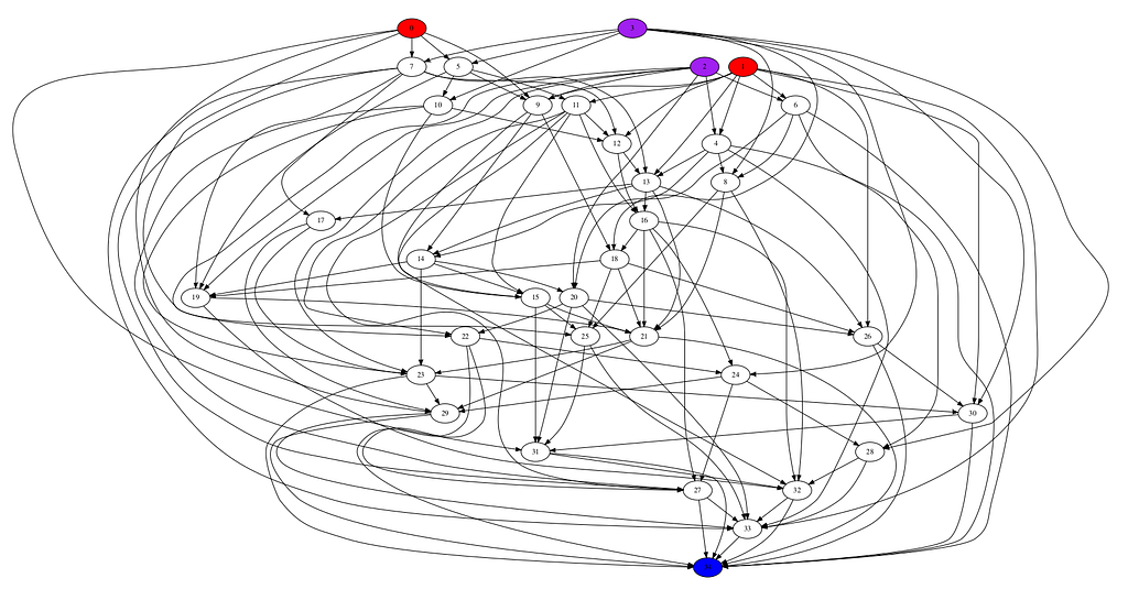
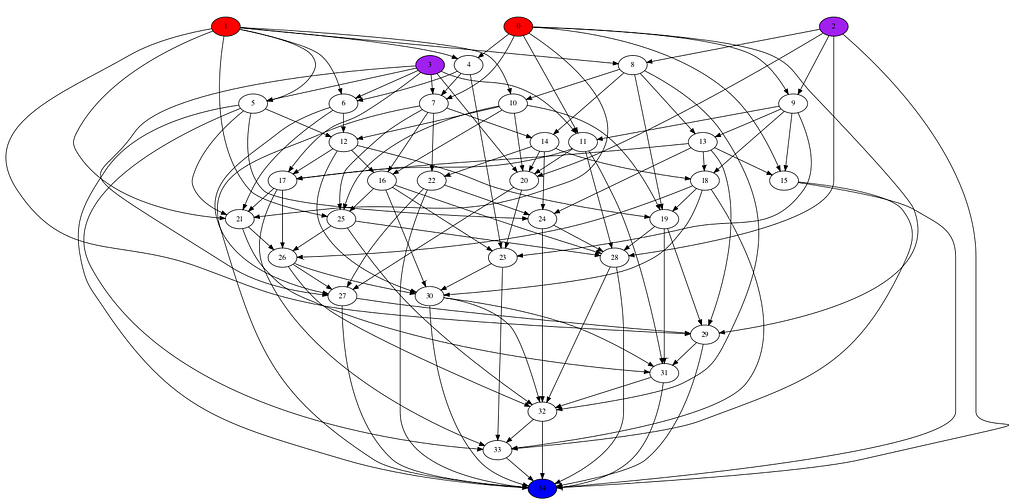
Without further ado lets apply a RWNN on a simple regression problem (sum of squares). Below (figure 1) a few RWNNs are presented; note that input (red) and bias (purple) nodes only have output connections, the output (blue) node only input connections and that the hidden nodes accept input connections only from nodes with smaller node-ids and output connections to nodes with bigger node-ids, hence representing feed forward RWNNs.

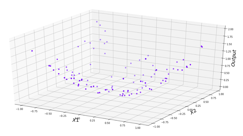
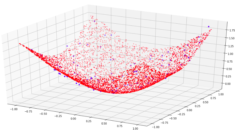
**Figure 1**: Architecture; 2 examples of RWNN with 2 input nodes (red) 2 bias nodes (purple) 1 output node (blue) and 30 hidden.

For the test case 100 random [x1,x2] input in [-1 ,1] are created their output is computed as x1²+x2² (Figure 2)

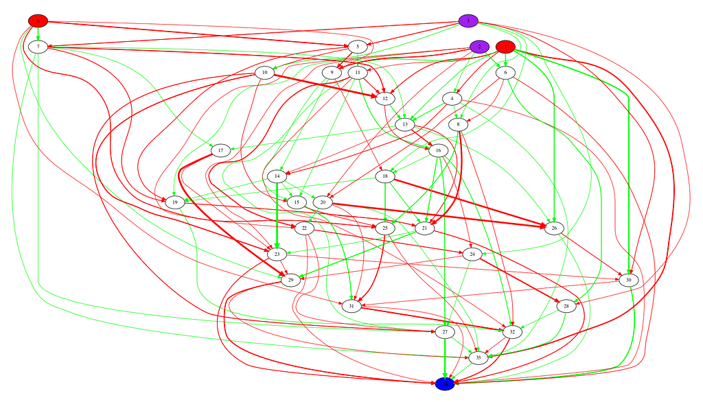
**Figure 2:** Training data; 100 random loci of the sum of squares function are used as training data for the toy example.

Using the good-old back propagation algorithm (Haykin, page 139 ) we can easily train our RWNN using our training data. Figure 3 presents the trained RWNN. Figure 4 the use of said trained RWNN on 5000 random test input points.

**Figure 3**: The Trained RWNN, width of synaptic connection is analogous to the absolute value of the associated weight. Red indicated negative weights and Green positive weights.

**Figure 4:** Test of trained RWNN on 500 random test points. Red are the test point predictions; Blue are the training points.

Epilogue

We’ve seen that we can indeed create RWNNs and train them to approximate a general function using error back propagation. Beacuse the generated RWNN are constrained to be feed forward neural networks no recurrence issues need to be addressed.
Next post will concerned with the use of an ensemble or RWNNs so as to quantify prediction uncertainty.